The City of Montreal recently began posting some crime records on their open data portal. For now, they’re only publishing data about break-ins, but it’s nonetheless a good occasion to play around with some of the new clustering features slated to be released in the next version of PostGIS.
PostGIS 2.3 will include functions to perform cluster analysis using two algorithms: k-means and DBSCAN (density-based spatial cluster of applications with noise). Here’s a bit of a worked example showing how to experiment with DBSCAN clustering in PostGIS using the Montreal data.
Loading the Data
First, we’ll download the data in CSV format:
wget http://donnees.ville.montreal.qc.ca/dataset/5829b5b0-ea6f-476f-be94-bc2b8797769a/resource/c6f482bf-bf0f-4960-8b2f-9982c211addd/download/interventionscitoyendo.csvAnd get a Postgres table ready to hold it:
1
2
3
4
5
6
7
8
9
10
CREATE TABLE mtl_crimes (
categorie text,
date date,
quart text,
pdq text,
x float,
y float,
lat float,
lon float
);
Now, we can load the data in:
1
\copy mtl_crimes FROM ~/Downloads/interventionscitoyendo.csv WITH CSV HEADER;
Remove some non-spatial records:
1
DELETE FROM mtl_crimes WHERE x=0;
And make a proper geometry column:
1
2
3
ALTER TABLE mtl_crimes ADD COLUMN geom geometry(Point, 2950);
UPDATE mtl_crimes SET geom = ST_SetSRID(ST_MakePoint(x, y), 2950);
CREATE INDEX ON mtl_crimes USING GIST(geom);
The coordinates were provided in both EPSG:2950, which is meter-based, and latitude/longitude. We’ll use the projected coordinates so that we can perform our analysis in meters (ST_ClusterDBSCAN doesn’t compute distances between geographic coordinates).
For good measure, we’ll also add an ID:
1
ALTER TABLE mtl_crimes ADD COLUMN id serial PRIMARY KEY;
Using ST_ClusterDBSCAN
Unlike k-means clustering, DBSCAN doesn’t require you to know the number of clusters beforehand. Instead, it requires you to specify the following two parameters:
- A distance tolerance, typically referred to as eps, and
- A density tolerance, typically referred to as minPoints.
To be included in a cluster, a geometry must be within eps distance of at least minPoints other geometries. Note that while PostGIS also uses the conventional name minPoints for the density tolerance, clusters can be formed from any 2D geometry type: (Multi)Points, (Multi)LineStrings, and (Multi)Polygons, including mixtures of these types and their curved variants.
The ST_ClusterIntersecting and ST_ClusterWithin functions in PostGIS 2.2 are really just special cases of DBSCAN clustering:
- For ST_ClusterIntersecting, eps = 0 and minPoints = 1
- For ST_ClusterWithin, eps is the tolerance specified by the user, and minPoints = 1
ST_ClusterDBSCAN is a windowing function that assigns a numeric cluster ID to each row in its partition.
1
2
3
4
5
6
7
8
9
10
11
12
13
14
15
SELECT id, ST_ClusterDBSCAN(geom, eps := 300, minPoints := 5)
OVER(ORDER BY id) AS cluster_id FROM mtl_crimes
LIMIT 8;
id | cluster_id
----+------------
1 |
2 |
3 | 6
4 | 14
5 | 11
6 | 4
7 | 4
8 | 4
(8 rows)
Here, we can see that point IDs 1 and 2 have a NULL cluster id; that is, they were not within 300 meters of at least five other points, so they were considered noise and not assigned to any cluster. Note that the ORDER BY id bit above doesn’t affect the clustering itself; it just puts the inputs into a predictable order so that the output is deterministic.
As with a GROUP BY clause used with an aggregate function, windowing functions allow us to divide our data into subsets that are processed independently. For example, we might want to independently process crimes depending on the time of day:
1
2
3
4
5
6
7
8
9
10
11
12
13
14
15
16
17
18
19
20
21
22
23
24
25
26
27
28
29
30
31
SELECT * FROM
(SELECT id, quart, ST_ClusterDBSCAN(geom, eps := 300, minPoints := 5)
OVER (PARTITION BY quart ORDER BY id) AS cluster_id
FROM mtl_crimes) sq
WHERE cluster_id = 4;
id | quart | cluster_id
-------+-------+------------
159 | jour | 4
4155 | jour | 4
4559 | jour | 4
7146 | jour | 4
9737 | jour | 4
9739 | jour | 4
10135 | jour | 4
175 | nuit | 4
5035 | nuit | 4
6502 | nuit | 4
7275 | nuit | 4
7939 | nuit | 4
9443 | nuit | 4
39 | soir | 4
184 | soir | 4
6305 | soir | 4
6594 | soir | 4
7705 | soir | 4
9068 | soir | 4
9449 | soir | 4
9498 | soir | 4
10362 | soir | 4
(22 rows)
Note that in this case, we have three unrelated clusters with ID 4. The generated cluster_id is unique only within its partition.
How many clusters do we have, anyway?
1
2
3
4
5
6
7
8
SELECT count(DISTINCT cluster_id) FROM
(SELECT ST_ClusterDBSCAN(geom, eps := 300, minPoints := 5)
OVER () AS cluster_id
FROM mtl_crimes) sq;
count
-------
101
(1 row)
That’s quite a few. Maybe we should tighten up our tolerance for what constitutes a hotspot of burglary. This is nearly 18 months of data, after all. How about break-ins that are within 300 meters of 15 other break-ins?
1
2
3
4
5
6
7
8
SELECT count(DISTINCT cluster_id) FROM
(SELECT ST_ClusterDBSCAN(geom, eps := 300, minPoints := 15)
OVER () AS cluster_id
FROM mtl_crimes) sq;
count
-------
66
(1 row)
Fifty other break-ins?
1
2
3
4
5
6
7
8
SELECT count(DISTINCT cluster_id) FROM
(SELECT ST_ClusterDBSCAN(geom, eps := 300, minPoints := 50)
OVER () AS cluster_id
FROM mtl_crimes) sq;
count
-------
15
(1 row)
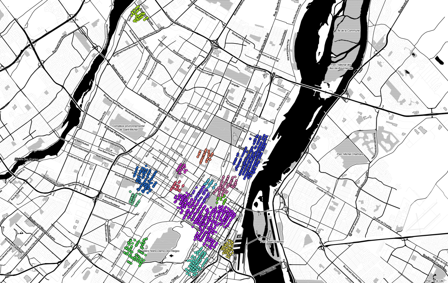
This seems like a reasonable number of clusters for us to look at. Let’s add the geometry column into the query, filter out the noise (cluster_id IS NULL) and plot it up in QGIS:
1
2
3
4
5
SELECT * FROM
(SELECT id, ST_ClusterDBSCAN(geom, eps := 300, minPoints := 50)
OVER () AS cluster_id, geom
FROM mtl_crimes) sq
WHERE cluster_id IS NOT NULL;